Training from timeseries CSV data
Working on timeseries allow to predict signals while taking into account the full history of inputs.
There are several use cases :
Model Surrogating: the timeseries consist in inputs and outputs of some physical system to model (or some model to surrogate)Predictive Maintenance/Prognostic: inputs are the observations of a system, output is the estimated remaining useful like, or estimated time to failureAnomaly Detection: inputs consist in observations at some time, outputs are predictions, i.e. the same observations but in the future. If real observations are different from predictions, then are some chances of presence of some anomaly.
The following tutorial describes a predictive maintenance case using data from https://ti.arc.nasa.gov/c/6/ and a recurrent neural network.
Data format
During data preparation, timeseries have to be separated using one CSV file per time serie.
Example seq_0.csv:
time;val1;val2;val3;val4; ... ;RUL
1.0;-0.0007;-0.0004;100.0;518.67; ... ;191
2.0;0.0019;-0.0003;100.0;518.67; ... ;190
3.0;-0.0043;0.0003;100.0;518.67; ... ;189
4.0;0.0007;0.0;100.0;518.67; ... ;188
...
192.0;0.0009;-0.0;100.0;518.67; ... ;0
CSV files should be split in training and test sets into different directories, and we recommend:
- to separate a predict set that will be used for final human check (it can be a subset of the test set)
- inside train and test directories, to separate time series by setups / parameters sets / experiments. This help to be sure to use very different series from train set in test set. If not doing so, the test set has a very large chance to be very similar to the train set, missing generalization assessment objectives.
Example file organization
$workdir/rawdata
$workdir/train/experiment_1/seq_0.csv
$workdir/train/experiment_1/seq_1.csv
$workdir/train/experiment_2/seq_0.csv
...
$workdir/test/experiment_5/seq_0.csv
$workdir/test/experiment_5/seq_1.csv
...
$workdir/predict/experiment_10/seq_0.csv
$workdir/predict/experiment_10/seq_1.csv
...
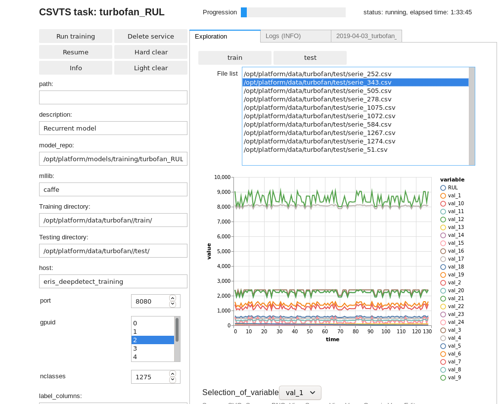
DD platform comes with a custom Jupyter UI that allows testing your timeseries dataset prior to training:
Training a timeseries model
Below, we train a model that takes a time-serie and predicts three output signals (columns 22, 23 and 24), as well as the remaining useful like value (RUL). This is a typical multi-valued regression job on time-series, that uses a recurrent neural network.
Using the DD platform, from a JupyterLab notebook, you can use
Timeseries notebook snippet:
turbofan_ts_model = CSVTS(
    "turbofan_RUL",
    host='deepdetect_training',
    port=8080,
    training_repo="/opt/platform/examples/turbofan/train/",
    testing_repo="/opt/platform/examples/turbofan/test/",
    model_repo="/opt/platform/models/training/turbofan_RUL",
    label_columns=["val_22","val_23","val_24","RUL"],
    ignore_columns=["time"],
    layers=["L100", "L100"],
    csv_separator=";",
    timesteps=100,
    gpuid=0,
    base_lr=0.0001,
    solver_type='RMSPROP',
    test_interval=500,
    iterations=1000000
)
turbofan_ts_model
This prepares for training a timeseries model with the following parameters:
turbofan_RULis the example job name
training_repospecifies the location of the train data
testing_repospecifies the location of the test data
label_columnsspecifies the name of the columns that will be considered as output at every timesteps. In the example, the model will use columnsval_1toval_21as input at every timestep and will be able to predictval_22,val_23,val_24andRULat every timestep.ignore_columnsspecifies the name of columns no to take into account in the model. Typically, the timestamptimeis to be ignored.layersspecifies a stacked LSTM architecture.["L100", "L100"]asks for 2 layers of LSTM with a memory/output size of 100. An affine transform will be automatically applied to have the desired output size (4 per timestep in this case). Another example is["L20","A10","L20","A3"]. This will instantiate an LSTM layer of memory/output size of 20, followed by an affine dimensionality reduction to 10 outputs, then another LSTM layer with memory/output size of 20 and another dimensionality reduction to have 3 outputs per timesteps (another “A4” will be automatically added in order to obtain the 4 outputs).cvs_separatorspecifies the separator used in data files.timestepsspecifies the length of series that will be generated from dataset to feed the network during the training phase. In the example, no dependencies on histories larger than 100 timesteps will be learned.gpuidspecifies with GPU to use, starting with number 0.base_lris the start learning rate of the optimizer. For general timeseries models, 1e-4 gives good results.solver_typespecifies the optimizer, see https://deepdetect.com/api/#launch-a-training-job andsolver_typefor the many optionstest_intervalis the number of iterations between two test measures.iterationsis the number of iterations asked for the training task.